Introduction

这是我大二暑假写的变分自编码器（VAE）学习笔记，主要参考 Kingma 和 Welling 的 An Introduction to Variational Autoencoders。原文用 Typst 排版，网页版由 Typst 源码借助 Gemini 转换，之后做过修订。原版 PDF 见下面的链接。

Motivation

机器学习模型大致可以分成判别模型和生成模型。判别模型学习从观测到预测目标的映射；生成模型则学习所有变量的联合分布。

生成模型描述的是数据在现实中如何产生。科学中的建模大多也是这个意思：提出关于生成过程的理论，再用观测去检验。气象学家用偏微分方程描述天气背后的物理过程，生物学家、化学家、经济学家也是类似的做法。

理解数据的生成过程还有一个好处：它往往对应因果关系，而因果关系比单纯的相关性更容易推广到新情况。

生成模型也可以用来做判别。用贝叶斯公式，可以把生成模型给出的联合分布转换成分类所需的条件概率。

两者的方向是相反的。以图像为例，可以设想现实中的图像是这样产生的：先有物体，生成三维形状，再投影到像素网格上。判别模型则反过来，直接把像素作为输入，映射到标签。

生成模型通常比判别模型对数据做出更强的假设。假设不准确时（实际中几乎总会有一些偏差），生成模型会有更大的渐近偏差。所以，如果目标只是判别，而且数据足够多，纯判别模型通常错误更少。但在数据有限时，生成模型可以帮助训练判别器。比如半监督学习中，标注样本很少而未标注样本很多，这时可以用数据的生成模型来改进分类。

更一般地说，学习生成过程可以得到对世界的有用抽象，这些抽象能服务于多个下游任务。寻找数据中解耦的、有语义的、统计独立的变化因素，通常称为无监督表示学习，VAE 在这方面被广泛使用。也可以把它看成一种隐式正则化：要求表示能解释数据的生成过程，就约束了从输入到表示的映射。

VAE 由两个耦合、但分别参数化的模型组成：编码器（识别模型）和解码器（生成模型）。识别模型为生成模型提供后验分布的近似，生成模型在类似"期望最大化"的迭代中用它来更新参数。反过来，生成模型为识别模型提供了学习有意义表示的框架。按贝叶斯公式，识别模型可以看作生成模型的近似逆。

与传统变分推断（VI）相比，VAE 的识别模型是输入的一个（随机）函数。传统 VI 给每个数据点单独设一个变分分布，大数据集上效率很低。识别模型用一组共享参数刻画输入与潜变量之间的关系，这称为摊销推断（amortized inference）。识别模型可以很复杂，但推断只需要一次前向计算，所以仍然很快。代价是采样会给梯度引入噪声。

VAE 框架最重要的贡献可能是重参数化技巧：一种重新组织梯度计算的简单方法，可以降低梯度估计的方差。

Aim

VAE 提供了一种有原则的方法：用随机梯度下降，同时学习深度潜变量模型和对应的推断模型。它在生成建模、半监督学习和表示学习中都有广泛应用。

Probabilistic Models and Variational Inference

概率模型中有未知量，而数据通常不足以完全确定它们，所以需要用（条件）概率分布来描述这种不确定性。最完整的概率模型是给出模型中所有变量的联合分布，它刻画了变量之间所有的相关和高阶依赖。

用 $\mathbf{x}$ 表示所有观测变量组成的向量，我们希望对它的联合分布建模。（这里把观测变量展平、拼接成一个向量。）

假设 $\mathbf{x}$ 是某个未知过程产生的随机样本，真实分布 $p^*(\mathbf{x})$ 未知。我们用一个参数为 $\theta$ 的模型 $p_\theta(\mathbf{x})$ 来近似它：

$$\begin{equation} \mathbf{x} \sim p_\theta(\mathbf{x}) \end{equation}$$

学习就是寻找参数 $\theta$，使模型分布尽量接近真实分布：

$$\begin{equation} p_\theta(\mathbf{x}) \approx p^*(\mathbf{x}) \end{equation}$$

Conditional Models

分类或回归问题关心的不是无条件模型 $p_\theta(\mathbf{x})$，而是条件模型 $p_\theta(y|\mathbf{x})$，它近似真实的条件分布 $p^*(y|\mathbf{x})$，即给定观测 $\mathbf{x}$ 时 $y$ 的分布。这时 $\mathbf{x}$ 称为模型的输入。和无条件情形一样，我们选择并优化模型，使得对任意 $\mathbf{x}$ 和 $y$：

$$\begin{equation} p_\theta(y|\mathbf{x}) \approx p^*(y|\mathbf{x}) \end{equation}$$

Directed Graphical Models and Neural Networks

我们使用有向概率图模型，也就是贝叶斯网络。其中所有变量组成一个有向无环图，联合分布分解为每个变量在其父节点条件下的分布的乘积：

$$\begin{equation} p_\theta(\mathbf{x}_1, ..., \mathbf{x}_M) = \prod_{j=1}^{M} p_\theta(\mathbf{x}_j | Pa(\mathbf{x}_j)) \end{equation}$$

$Pa(\mathbf{x}_j)$ 是节点 $j$ 在图中的父节点集合。没有父节点的变量，条件分布就是它的先验。各个条件分布可以用神经网络参数化。

Dataset

数据集 $\mathcal{D}$ 由 $N \ge 1$ 个数据点组成：

$$\begin{equation} \mathcal{D} = \{\mathbf{x}^{(1)}, \mathbf{x}^{(2)}, ..., \mathbf{x}^{(N)}\} \equiv \{\mathbf{x}^{(i)}\}_{i=1}^N \equiv \mathbf{x}^{(1:N)} \end{equation}$$

假设数据点是同一个系统的独立测量，即独立同分布（i.i.d.）。在给定参数的条件下，数据集的概率等于各数据点概率的乘积，对数概率为：

$$\begin{equation} \log p_\theta(\mathcal{D}) = \sum_{\mathbf{x} \in \mathcal{D}} \log p_\theta(\mathbf{x}) \end{equation}$$

Maximum Likelihood and Minibatch SGD

最常用的训练准则是最大对数似然。最大化对数似然等价于最小化数据分布与模型分布之间的 KL 散度。常用的优化方法是随机梯度下降（SGD）。

数据集很大时，每一步都用全部数据计算梯度太贵。做法是随机抽一个大小为 $N_\mathcal{M}$ 的小批量 $\mathcal{M}$，在它上面算梯度。我们需要这个梯度在期望上等于全数据集上的梯度。

全数据集和小批量的对数似然分别是：

$$\begin{equation} \log p_\theta(\mathcal{D}) = \sum_{\mathbf{x} \in \mathcal{D}} \log p_\theta(\mathbf{x}), \qquad \log p_\theta(\mathcal{M}) = \sum_{\mathbf{x} \in \mathcal{M}} \log p_\theta(\mathbf{x}) \end{equation}$$

按每个数据点平均后，小批量给出全数据集平均对数似然的无偏估计，梯度也是如此：

$$\begin{equation} \frac{1}{N} \log p_\theta(\mathcal{D}) \approx \frac{1}{N_\mathcal{M}} \log p_\theta(\mathcal{M}) = \frac{1}{N_\mathcal{M}} \sum_{\mathbf{x} \in \mathcal{M}} \log p_\theta(\mathbf{x}) \end{equation}$$ $$\begin{equation} \frac{1}{N} \nabla_\theta \log p_\theta(\mathcal{D}) \approx \frac{1}{N_\mathcal{M}} \nabla_\theta \log p_\theta(\mathcal{M}) = \frac{1}{N_\mathcal{M}} \sum_{\mathbf{x} \in \mathcal{M}} \nabla_\theta \log p_\theta(\mathbf{x}) \end{equation}$$

小批量梯度的无偏性

下面验证这一点。全数据集的梯度是：

$$\begin{equation} \nabla_\theta \log p_\theta(\mathcal{D}) = \sum_{i=1}^N \nabla_\theta \log p_\theta(\mathbf{x}_i) \end{equation}$$

小批量只有 $N_\mathcal{M}$ 个点，要估计全数据集的梯度（而不是平均梯度），需要乘以比例 $\frac{N}{N_\mathcal{M}}$ 来补偿样本数的差异：

$$\begin{equation} \tilde{\nabla}_\theta \log p_\theta(\mathcal{M}) = \frac{N}{N_\mathcal{M}} \sum_{j=1}^{N_\mathcal{M}} \nabla_\theta \log p_\theta(\mathbf{x}_j) \end{equation}$$

每个 $\mathbf{x}_j$ 都是从 $\mathcal{D}$ 中均匀随机抽取的，所以：

$$\begin{align} \mathbb{E}[\tilde{\nabla}_\theta \log p_\theta(\mathcal{M})] &= \frac{N}{N_\mathcal{M}} \mathbb{E}\left[\sum_{j=1}^{N_\mathcal{M}} \nabla_\theta \log p_\theta(\mathbf{x}_j)\right] \\ &= \frac{N}{N_\mathcal{M}} N_\mathcal{M} \, \mathbb{E}[\nabla_\theta \log p_\theta(\mathbf{x})] \\ &= N \, \mathbb{E}[\nabla_\theta \log p_\theta(\mathbf{x})] \end{align}$$

而均匀抽取一个点的期望梯度就是全数据集梯度的平均值：

$$\begin{equation} N \, \mathbb{E}[\nabla_\theta \log p_\theta(\mathbf{x})] = \sum_{i=1}^N \nabla_\theta \log p_\theta(\mathbf{x}_i) = \nabla_\theta \log p_\theta(\mathcal{D}) \end{equation}$$

所以乘以 $\frac{N}{N_\mathcal{M}}$ 之后，小批量梯度是全数据集梯度的无偏估计。实践中通常直接用平均形式，两者只差一个常数倍，可以并入学习率。

Learning and Inference in Deep Latent Variable Models

Latent Variables

可以把上面的全观测有向模型扩展到含潜变量的情形。潜变量是模型的一部分，但没有被观测到，不在数据集里，通常记作 $\mathbf{z}$。对观测变量 $\mathbf{x}$ 建模时，有向图模型表示的是 $\mathbf{x}$ 和 $\mathbf{z}$ 的联合分布 $p_\theta(\mathbf{x}, \mathbf{z})$。$\mathbf{x}$ 的边缘分布为：

$$\begin{equation} p_\theta(\mathbf{x}) = \int p_\theta(\mathbf{x}, \mathbf{z}) \, d\mathbf{z} \end{equation}$$

把它看作 $\theta$ 的函数时，称为（单个数据点的）边缘似然或模型证据。

这种隐式定义的分布可以很灵活。如果 $\mathbf{z}$ 是离散的，$p_\theta(\mathbf{x}|\mathbf{z})$ 是高斯分布，那么 $p_\theta(\mathbf{x})$ 就是高斯混合。如果 $\mathbf{z}$ 连续，$p_\theta(\mathbf{x})$ 可以看作无穷多个分量的混合，表达能力可能比离散混合更强。这样的边缘分布也叫复合概率分布。

Deep Latent Variable Models

深度潜变量模型（deep latent variable model, DLVM）指分布由神经网络参数化的潜变量模型 $p_\theta(\mathbf{x}, \mathbf{z})$，也可以带上条件，如 $p_\theta(\mathbf{x}, \mathbf{z} | \mathbf{y})$。它的一个重要优点是：即使每个因子（先验或条件分布）都比较简单，比如条件高斯，边缘分布 $p_\theta(\mathbf{x})$ 也可以非常复杂，几乎能包含任意依赖关系。这让 DLVM 适合用来近似复杂的真实分布 $p^*(\mathbf{x})$。

最简单、也最常见的 DLVM 是这样分解的：

$$\begin{equation} p_\theta(\mathbf{x}, \mathbf{z}) = p_\theta(\mathbf{z}) p_\theta(\mathbf{x}|\mathbf{z}) \end{equation}$$

$p_\theta(\mathbf{z})$ 和 $p_\theta(\mathbf{x}|\mathbf{z})$ 的形式由我们指定。$p(\mathbf{z})$ 不依赖任何观测，称为潜变量的先验分布。

DLVM 的困难在于，边缘似然 $p_\theta(\mathbf{x})$ 和后验 $p_\theta(\mathbf{z}|\mathbf{x}) = p_\theta(\mathbf{x}, \mathbf{z}) / p_\theta(\mathbf{x})$ 一般都没有解析形式，无法直接计算和优化。VAE 就是为了解决这个问题。

Variational Autoencoders

Encoder or Approximate Posterior

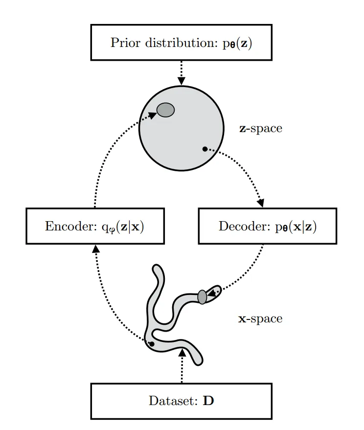
VAE 框架提供了一种高效的方法，用 SGD 同时优化 DLVM 和对应的推断模型。为了让后验推断和学习变得可处理，引入一个带参数的推断模型 $q_\phi(\mathbf{z}|\mathbf{x})$，也称为编码器或识别模型。$\phi$ 是它的参数，称为变分参数。我们优化 $\phi$，使得：

$$\begin{equation} q_\phi(\mathbf{z}|\mathbf{x}) \approx p_\theta(\mathbf{z}|\mathbf{x}) \end{equation}$$

和 DLVM 一样，推断模型可以是（几乎）任意的有向图模型：

$$\begin{equation} q_\phi(\mathbf{z}|\mathbf{x}) = q_\phi(\mathbf{z}_1, ..., \mathbf{z}_M | \mathbf{x}) = \prod_{j=1}^{M} q_\phi(\mathbf{z}_j | Pa(\mathbf{z}_j), \mathbf{x}) \end{equation}$$

$Pa(\mathbf{z}_j)$ 是 $\mathbf{z}_j$ 在图中的父变量集合。$q_\phi(\mathbf{z}|\mathbf{x})$ 同样可以用深度神经网络参数化，例如：

$$\begin{equation} (\mu, \log\sigma) = \text{EncoderNeuralNet}_\phi(\mathbf{x}) \end{equation}$$ $$\begin{equation} q_\phi(\mathbf{z}|\mathbf{x}) = \mathcal{N}(\mathbf{z}; \mu, \text{diag}(\sigma^2)) \end{equation}$$

数据集中所有数据点共用同一个编码器做后验推断。这和传统变分推断不同：后者的变分参数不共享，需要对每个数据点单独迭代优化。摊销推断省去了每个数据点的优化循环，也能充分利用 SGD 的效率。

Evidence Lower Bound (ELBO)

VAE 通过编码器和解码器，结合先验、近似后验和重建分布，对复杂的数据分布进行建模和生成。

对任意推断模型 $q_\phi(\mathbf{z}|\mathbf{x})$，对数似然可以分解为：

$$\begin{align} \log p_\theta(\mathbf{x}) &= \mathbb{E}_{q_\phi(\mathbf{z}|\mathbf{x})} [\log p_\theta(\mathbf{x})] \\ &= \mathbb{E}_{q_\phi(\mathbf{z}|\mathbf{x})} \left[\log \frac{p_\theta(\mathbf{x},\mathbf{z})}{p_\theta(\mathbf{z}|\mathbf{x})}\right] \\ &= \mathbb{E}_{q_\phi(\mathbf{z}|\mathbf{x})} \left[\log \frac{p_\theta(\mathbf{x},\mathbf{z})}{q_\phi(\mathbf{z}|\mathbf{x})} \frac{q_\phi(\mathbf{z}|\mathbf{x})}{p_\theta(\mathbf{z}|\mathbf{x})}\right] \\ &= \underbrace{\mathbb{E}_{q_\phi(\mathbf{z}|\mathbf{x})} \left[\log \frac{p_\theta(\mathbf{x},\mathbf{z})}{q_\phi(\mathbf{z}|\mathbf{x})}\right]}_{\mathcal{L}_{\theta, \phi}(\mathbf{x}) \text{ ("ELBO")}} + \underbrace{\mathbb{E}_{q_\phi(\mathbf{z}|\mathbf{x})} \left[\log \frac{q_\phi(\mathbf{z}|\mathbf{x})}{p_\theta(\mathbf{z}|\mathbf{x})}\right]}_{D_{\text{KL}}(q_\phi(\mathbf{z}|\mathbf{x}) || p_\theta(\mathbf{z}|\mathbf{x}))} \end{align}$$

第二项是 $q_\phi(\mathbf{z}|\mathbf{x})$ 与真实后验 $p_\theta(\mathbf{z}|\mathbf{x})$ 之间的 KL 散度。它非负，并且当且仅当 $q_\phi(\mathbf{z}|\mathbf{x})$ 等于真实后验时为零：

$$\begin{equation} D_{\text{KL}}(q_\phi(\mathbf{z}|\mathbf{x}) || p_\theta(\mathbf{z}|\mathbf{x})) \ge 0 \end{equation}$$

第一项称为变分下界，或证据下界（ELBO）：

$$\begin{equation} \mathcal{L}_{\theta,\phi}(\mathbf{x}) = \mathbb{E}_{q_\phi(\mathbf{z}|\mathbf{x})} [\log p_\theta(\mathbf{x},\mathbf{z}) - \log q_\phi(\mathbf{z}|\mathbf{x})] \end{equation}$$

由于 KL 散度非负，ELBO 是对数似然的下界：

$$\begin{align} \mathcal{L}_{\theta,\phi}(\mathbf{x}) &= \log p_\theta(\mathbf{x}) - D_{\text{KL}}(q_\phi(\mathbf{z}|\mathbf{x}) || p_\theta(\mathbf{z}|\mathbf{x})) \\ &\le \log p_\theta(\mathbf{x}) \end{align}$$

这个分解说明，最大化 ELBO 同时做了两件事：提高对数似然，让生成模型变好；缩小 KL 散度，让推断模型更接近真实后验。

Stochastic Gradient-Based Optimization of the ELBO

ELBO 的一个重要性质是，可以用 SGD 对所有参数（$\phi$ 和 $\theta$）联合优化。从随机初始化开始，不断更新直到收敛。数据集上的目标是各个数据点 ELBO 之和：

$$\begin{equation} \mathcal{L}_{\theta, \phi}(\mathcal{D}) = \sum_{\mathbf{x} \in \mathcal{D}} \mathcal{L}_{\theta, \phi}(\mathbf{x}) \end{equation}$$

一般来说，单个数据点的 ELBO 及其梯度 $\nabla_{\theta,\phi} \mathcal{L}_{\theta,\phi}(\mathbf{x})$ 无法精确计算。但它们有好的无偏估计量 $\tilde{\nabla}_{\theta,\phi}\mathcal{L}_{\theta,\phi}(\mathbf{x})$，所以仍然可以做小批量 SGD。对生成模型参数 $\theta$，无偏梯度很容易得到，因为期望的分布不依赖 $\theta$：

$$\begin{align} \nabla_{\theta} \mathcal{L}_{\theta, \phi}(\mathbf{x}) &= \nabla_{\theta} \mathbb{E}_{q_{\phi}(\mathbf{z}|\mathbf{x})} [\log p_{\theta}(\mathbf{x}, \mathbf{z}) - \log q_{\phi}(\mathbf{z}|\mathbf{x})] \\ &= \mathbb{E}_{q_{\phi}(\mathbf{z}|\mathbf{x})} [\nabla_{\theta}(\log p_{\theta}(\mathbf{x}, \mathbf{z}) - \log q_{\phi}(\mathbf{z}|\mathbf{x}))] \\ &\approx \nabla_{\theta}(\log p_{\theta}(\mathbf{x}, \mathbf{z}) - \log q_{\phi}(\mathbf{z}|\mathbf{x})) \\ &= \nabla_{\theta}\log p_{\theta}(\mathbf{x}, \mathbf{z}) \end{align}$$

倒数第二行是用一个样本 $\mathbf{z} \sim q_\phi(\mathbf{z}|\mathbf{x})$ 做的蒙特卡罗估计。对变分参数 $\phi$ 就没这么简单了：期望本身是在 $q_\phi$ 下取的，依赖 $\phi$，不能直接把梯度移进期望里。这正是重参数化技巧要解决的问题。

Reparameterization Trick

对连续潜变量，并且编码器和生成模型都可微时，可以通过变量替换直接对 ELBO 关于 $\phi$ 和 $\theta$ 求导，这称为重参数化技巧。

Change of variables

首先，把随机变量 $\mathbf{z} \sim q_{\phi}(\mathbf{z}|\mathbf{x})$ 写成另一个随机变量 $\epsilon$ 在给定 $\mathbf{x}$ 和 $\phi$ 下的可微（可逆）变换：

$$\begin{equation} \mathbf{z} = g(\epsilon, \phi, \mathbf{x}) \end{equation}$$

其中 $\epsilon$ 的分布与 $\mathbf{x}$ 和 $\phi$ 都无关。这样，随机性全部来自 $\epsilon$，而 $\mathbf{z}$ 对 $\phi$ 是可微的，梯度可以穿过采样过程反向传播。

Algorithm 1: ELBO 的随机优化。噪声既来自小批量采样，也来自 $p(\epsilon)$ 的采样，因此这是一个双重随机的优化过程。这个算法也称为自编码变分贝叶斯（Auto-Encoding Variational Bayes, AEVB）。

Data:

• $\mathcal{D}$: Dataset
• $q_\phi(\mathbf{z}|\mathbf{x})$: Inference model
• $p_\theta(\mathbf{x},\mathbf{z})$: Generative model

Result:

• $\theta, \phi$: Learned parameters

---

$(\theta, \phi) \leftarrow$ Initialize parameters

while SGD not converged do

     $\mathcal{M} \sim \mathcal{D}$ (Random minibatch of data)

     $\epsilon \sim p(\epsilon)$ (Random noise for every datapoint in $\mathcal{M}$)

     Compute $\tilde{\mathcal{L}}_{\theta,\phi}(\mathcal{M},\epsilon)$ and its gradients $\nabla_{\theta,\phi} \tilde{\mathcal{L}}_{\theta,\phi}(\mathcal{M},\epsilon)$

     Update $\theta$ and $\phi$ using SGD optimizer

end

Gradient of expectation under change of variable

做了变量替换后，期望可以改写成关于 $\epsilon$ 的期望：

$$\begin{equation} \mathbb{E}_{q_{\phi}(\mathbf{z}|\mathbf{x})} [f(\mathbf{z})] = \mathbb{E}_{p(\epsilon)} [f(\mathbf{z})] \end{equation}$$

其中 $\mathbf{z}=g(\epsilon,\phi,\mathbf{x})$。现在期望的分布 $p(\epsilon)$ 不依赖 $\phi$，梯度和期望可以交换，再用从 $p(\epsilon)$ 采样的单个 $\epsilon$ 做蒙特卡罗估计：

$$\begin{align} \nabla_{\phi} \mathbb{E}_{q_{\phi}(\mathbf{z}|\mathbf{x})} [f(\mathbf{z})] &= \nabla_{\phi} \mathbb{E}_{p(\epsilon)} [f(\mathbf{z})] \\ &= \mathbb{E}_{p(\epsilon)} [\nabla_{\phi} f(\mathbf{z})] \\ &\approx \nabla_{\phi} f(\mathbf{z}) \end{align}$$

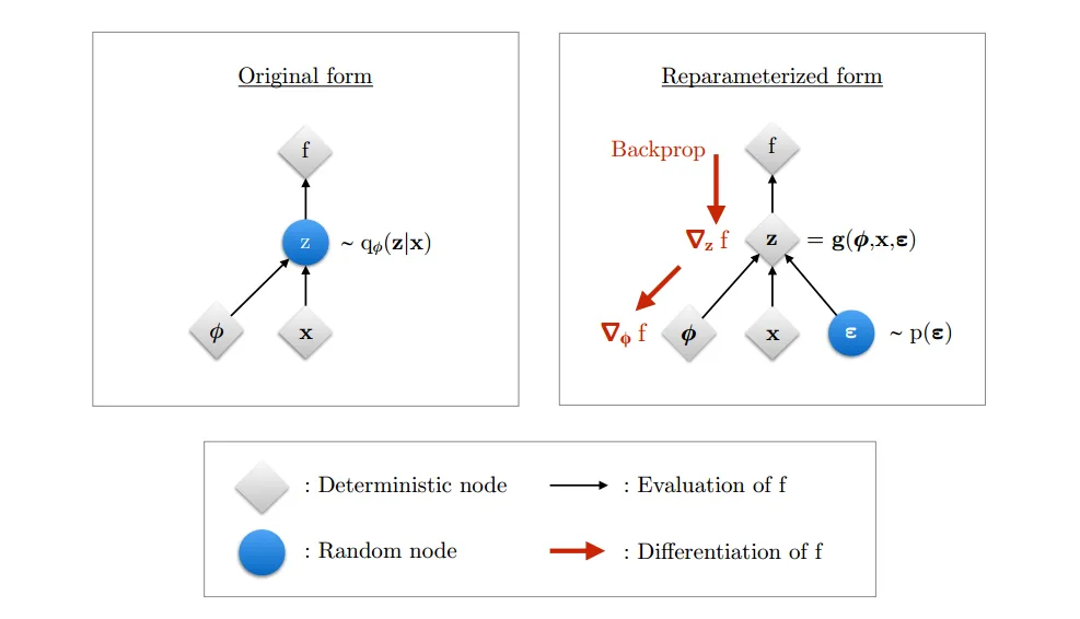
上图对比了原始形式和重参数化形式。

左图：原始形式。 灰色节点是确定性节点（如目标函数 $f$），蓝色节点是随机节点（如潜变量 $\mathbf{z}$）。$\mathbf{z}$ 从 $q_\phi(\mathbf{z}|\mathbf{x})$ 中采样，$f$ 依赖 $\mathbf{z}$。我们想对 $\phi$ 求梯度，但梯度无法穿过"采样"这一步反向传播。

右图：重参数化形式。 随机性被移到噪声 $\epsilon$ 上，$\epsilon$ 从简单分布 $p(\epsilon)$ 中采样，$\mathbf{z} = g(\phi, \mathbf{x}, \epsilon)$ 变成确定性节点。由于 $\mathbf{z}$ 是 $\phi$ 的可微函数，梯度可以沿 $f \to \mathbf{z} \to \phi$ 反向传播。

总结一下，重参数化分三步：

1. 变量替换：把 $\mathbf{z}$ 写成噪声、参数和输入的可微函数 $\mathbf{z} = g(\epsilon, \phi, \mathbf{x})$。
2. 改写期望：$\mathbb{E}_{q_\phi(\mathbf{z}|\mathbf{x})} [f(\mathbf{z})] = \mathbb{E}_{p(\epsilon)} [f(\mathbf{z})]$。
3. 计算梯度：交换梯度与期望，用蒙特卡罗采样估计。

这样就能用普通的反向传播计算梯度，而且得到的梯度估计方差通常比其他无偏估计（如 score function 估计）低得多。

Gradient of ELBO

用重参数化，把关于 $q_\phi(\mathbf{z}|\mathbf{x})$ 的期望换成关于 $p(\epsilon)$ 的期望，ELBO 可以写成：

$$\begin{align} \mathcal{L}_{\theta, \phi}(\mathbf{x}) &= \mathbb{E}_{q_{\phi}(\mathbf{z}|\mathbf{x})} [\log p_{\theta}(\mathbf{x}, \mathbf{z}) - \log q_{\phi}(\mathbf{z}|\mathbf{x})] \\ &= \mathbb{E}_{p(\epsilon)} [\log p_{\theta}(\mathbf{x}, \mathbf{z}) - \log q_{\phi}(\mathbf{z}|\mathbf{x})] \end{align}$$

于是可以用单个噪声样本构造单个数据点 ELBO 的蒙特卡罗估计 $\tilde{\mathcal{L}}_{\theta, \phi}(\mathbf{x})$：

$$\begin{align} \epsilon &\sim p(\epsilon) \\ \mathbf{z} &= g(\phi, \mathbf{x}, \epsilon) \\ \tilde{\mathcal{L}}_{\theta, \phi}(\mathbf{x}) &= \log p_{\theta}(\mathbf{x}, \mathbf{z}) - \log q_{\phi}(\mathbf{z}|\mathbf{x}) \end{align}$$

这一串运算可以在 PyTorch、TensorFlow 等框架里写成计算图，对 $\theta$ 和 $\phi$ 自动求导。

这个算法最初称为 AEVB 算法。更一般地，重参数化的 ELBO 估计称为随机梯度变分贝叶斯（SGVB）估计，它也可以用来估计模型参数的后验。

Computation of $\log q_\phi(\mathbf{z}|\mathbf{x})$

计算 ELBO 估计时，需要在给定 $\mathbf{x}$ 和 $\mathbf{z}$（或者等价地 $\epsilon$）时计算 $\log q_\phi(\mathbf{z}|\mathbf{x})$。只要变换 $g$ 选得合适，这一步很简单。

噪声分布 $p(\epsilon)$ 是我们自己选的，密度已知。只要 $g$ 可逆，$\epsilon$ 和 $\mathbf{z}$ 的密度有如下关系（推导见下一小节）：

$$\begin{equation} \log q_{\phi}(\mathbf{z}|\mathbf{x}) = \log p(\epsilon) - \log d_{\phi}(\mathbf{x}, \epsilon) \end{equation}$$

第二项是雅可比矩阵 $\frac{\partial \mathbf{z}}{\partial \epsilon}$ 行列式绝对值的对数：

$$\begin{equation} \log d_{\phi}(\mathbf{x}, \epsilon) = \log \left| \det\left(\frac{\partial \mathbf{z}}{\partial \epsilon}\right) \right| \end{equation}$$ $$\begin{equation} \frac{\partial \mathbf{z}}{\partial \epsilon} = \frac{\partial(z_1, ..., z_k)}{\partial(\epsilon_1, ..., \epsilon_k)} = \begin{pmatrix} \frac{\partial z_1}{\partial \epsilon_1} & \cdots & \frac{\partial z_1}{\partial \epsilon_k} \\ \vdots & \ddots & \vdots \\ \frac{\partial z_k}{\partial \epsilon_1} & \cdots & \frac{\partial z_k}{\partial \epsilon_k} \end{pmatrix} \end{equation}$$

推导

设 $\mathbf{z} = g(\epsilon, \phi, \mathbf{x})$，$g$ 可微且可逆。由概率密度的变量替换公式：

$$\begin{equation} q_{\phi}(\mathbf{z}|\mathbf{x}) = p(\epsilon) \left| \det\left(\frac{\partial \epsilon}{\partial \mathbf{z}}\right) \right| \end{equation}$$

我们通常知道的是 $\frac{\partial \mathbf{z}}{\partial \epsilon}$，而不是 $\frac{\partial \epsilon}{\partial \mathbf{z}}$。利用逆映射的雅可比行列式互为倒数：

$$\begin{equation} \left| \det\left(\frac{\partial \epsilon}{\partial \mathbf{z}}\right) \right| = \frac{1}{\left| \det\left(\frac{\partial \mathbf{z}}{\partial \epsilon}\right) \right|} \end{equation}$$

代入得到：

$$\begin{equation} q_{\phi}(\mathbf{z}|\mathbf{x}) = p(\epsilon) \left| \det\left(\frac{\partial \mathbf{z}}{\partial \epsilon}\right) \right|^{-1} \end{equation}$$

取对数就是上面的公式。

Factorized Gaussian posteriors

常见的选择是因子化高斯编码器：

$$\begin{equation} q_{\phi}(\mathbf{z}|\mathbf{x}) = \mathcal{N}(\mathbf{z}; \mu, \text{diag}(\sigma^2)) \end{equation}$$

其中 $\mu$ 和 $\log\sigma$ 由编码器网络给出：

$$\begin{equation} (\mu, \log\sigma) = \text{EncoderNeuralNet}_{\phi}(\mathbf{x}) \end{equation}$$

后验分解为每个潜变量各自的高斯分布的乘积：

$$\begin{equation} q_{\phi}(\mathbf{z}|\mathbf{x}) = \prod_i q_{\phi}(z_i|\mathbf{x}) = \prod_i \mathcal{N}(z_i; \mu_i, \sigma_i^2) \end{equation}$$

重参数化时，把 $\mathbf{z}$ 写成标准正态噪声 $\epsilon$ 的线性变换：

$$\begin{equation} \epsilon \sim \mathcal{N}(0, \mathbf{I}) \end{equation}$$ $$\begin{equation} \mathbf{z} = \mu + \sigma \odot \epsilon \end{equation}$$

从 $\epsilon$ 到 $\mathbf{z}$ 的雅可比矩阵是对角矩阵，对角元为 $\sigma$：

$$\begin{equation} \frac{\partial \mathbf{z}}{\partial \epsilon} = \text{diag}(\sigma) \end{equation}$$

对角矩阵的行列式是对角元之积，所以对数行列式是对角元的对数之和：

$$\begin{equation} \log d_{\phi}(\mathbf{x}, \epsilon) = \log \left| \det\left(\frac{\partial \mathbf{z}}{\partial \epsilon}\right) \right| = \sum_i \log \sigma_i \end{equation}$$

于是后验对数密度为：

$$\begin{align} \log q_{\phi}(\mathbf{z}|\mathbf{x}) &= \log p(\epsilon) - \log d_{\phi}(\mathbf{x}, \epsilon) \\ &= \sum_i \left( \log \mathcal{N}(\epsilon_i; 0, 1) - \log \sigma_i \right) \end{align}$$

Full-covariance Gaussian posterior

因子化高斯可以推广到全协方差高斯：

$$\begin{equation} q_{\phi}(\mathbf{z}|\mathbf{x}) = \mathcal{N}(\mathbf{z}; \mu, \Sigma) \end{equation}$$

对应的重参数化为：

$$\begin{align} \epsilon &\sim \mathcal{N}(0, \mathbf{I}) \\ \mathbf{z} &= \mu + \mathbf{L}\epsilon \end{align}$$

$\mathbf{L}$ 是对角元非零的下（或上）三角矩阵，非对角元刻画了 $\mathbf{z}$ 各分量之间的相关性。这样构造的 $\mathbf{z}$ 协方差正是 $\Sigma$：

$$\begin{equation} \Sigma = \mathbb{E}[(\mathbf{z} - \mu)(\mathbf{z} - \mu)^T] = \mathbb{E}[\mathbf{L}\epsilon \epsilon^T \mathbf{L}^T] = \mathbf{L}\,\mathbb{E}[\epsilon \epsilon^T]\,\mathbf{L}^T = \mathbf{L}\mathbf{L}^T \end{equation}$$

这里用到了 $\mathbb{E}[\epsilon \epsilon^T] = \mathbf{I}$。也就是说，$\mathbf{L}$ 是 $\Sigma$ 的 Cholesky 因子。雅可比矩阵很简单：

$$\begin{equation} \frac{\partial \mathbf{z}}{\partial \epsilon} = \mathbf{L} \end{equation}$$

三角矩阵的行列式等于对角元之积，所以：

$$\begin{equation} \log \left| \det\left(\frac{\partial \mathbf{z}}{\partial \epsilon}\right) \right| = \sum_i \log|L_{ii}| \end{equation}$$

后验对数密度为：

$$\begin{equation} \log q_{\phi}(\mathbf{z}|\mathbf{x}) = \log p(\epsilon) - \sum_i \log|L_{ii}| \end{equation}$$

实践中，可以让编码器同时输出 $\mu$、$\log\sigma$ 和一个矩阵 $\mathbf{L}'$：

$$\begin{equation} (\mu, \log\sigma, \mathbf{L}') \leftarrow \text{EncoderNeuralNet}_{\phi}(\mathbf{x}) \end{equation}$$

再这样构造 $\mathbf{L}$：

$$\begin{equation} \mathbf{L} \leftarrow \mathbf{L}_{\text{mask}} \odot \mathbf{L}' + \text{diag}(\sigma) \end{equation}$$

$\mathbf{L}_{\text{mask}}$ 是掩码矩阵，对角线以下的元素为 1，对角线及以上为 0。这样 $\mathbf{L}$ 一定是下三角矩阵，对角元就是 $\sigma$，因此对数行列式和因子化情形一样：

$$\begin{equation} \log \left| \det\left(\frac{\partial \mathbf{z}}{\partial \epsilon}\right) \right| = \sum_i \log \sigma_i \end{equation}$$

Algorithm 2: 计算单个数据点 ELBO 的无偏估计。例子中推断模型是全协方差高斯，生成模型是因子化伯努利分布。$\mathbf{L}_{\text{mask}}$ 是掩码矩阵，对角线及以上为 0，对角线以下为 1。

Data:

• $\mathbf{x}$: a datapoint, and optionally other conditioning information
• $\epsilon$: a random sample from $p(\epsilon) = \mathcal{N}(0,\mathbf{I})$
• $\theta$: Generative model parameters
• $\phi$: Inference model parameters
• $q_\phi(\mathbf{z}|\mathbf{x})$: Inference model
• $p_\theta(\mathbf{x},\mathbf{z})$: Generative model

Result:

• $\tilde{\mathcal{L}}$: 单个数据点 ELBO $\mathcal{L}_{\theta,\phi}(\mathbf{x})$ 的无偏估计

---

$(\mu, \log\sigma, \mathbf{L}') \leftarrow \text{EncoderNeuralNet}_\phi(\mathbf{x})$

$\mathbf{L} \leftarrow \mathbf{L}_{\text{mask}} \odot \mathbf{L}' + \text{diag}(\sigma)$

$\epsilon \sim \mathcal{N}(0,\mathbf{I})$

$\mathbf{z} \leftarrow \mathbf{L}\epsilon + \mu$

$\tilde{\mathcal{L}}_{\text{logqz}} \leftarrow -\sum_i \left(\frac{1}{2}(\epsilon_i^2 + \log(2\pi)) + \log\sigma_i\right)$ （即 $\log q_\phi(\mathbf{z}|\mathbf{x})$）

$\tilde{\mathcal{L}}_{\text{logpz}} \leftarrow -\sum_i \frac{1}{2}(z_i^2 + \log(2\pi))$ （即 $\log p_\theta(\mathbf{z})$）

$\mathbf{p} \leftarrow \text{DecoderNeuralNet}_\theta(\mathbf{z})$

$\tilde{\mathcal{L}}_{\text{logpx}} \leftarrow \sum_i \left(x_i \log p_i + (1 - x_i) \log(1 - p_i)\right)$ （即 $\log p_\theta(\mathbf{x}|\mathbf{z})$）

$\tilde{\mathcal{L}} = \tilde{\mathcal{L}}_{\text{logpx}} + \tilde{\mathcal{L}}_{\text{logpz}} - \tilde{\mathcal{L}}_{\text{logqz}}$

Estimation of the Marginal Likelihood

训练好 VAE 之后，可以用采样估计模型赋予数据的概率。单个数据点的边缘似然可以写成：

$$\begin{equation} \log p_{\theta}(\mathbf{x}) = \log \mathbb{E}_{q_{\phi}(\mathbf{z}|\mathbf{x})} \left[ \frac{p_{\theta}(\mathbf{x}, \mathbf{z})}{q_{\phi}(\mathbf{z}|\mathbf{x})} \right] \end{equation}$$

从 $q_\phi(\mathbf{z}|\mathbf{x})$ 采样 $L$ 次，得到蒙特卡罗估计：

$$\begin{equation} \log p_{\theta}(\mathbf{x}) \approx \log \left( \frac{1}{L} \sum_{l=1}^{L} \frac{p_{\theta}(\mathbf{x}, \mathbf{z}^{(l)})}{q_{\phi}(\mathbf{z}^{(l)}|\mathbf{x})} \right) \end{equation}$$

每个 $\mathbf{z}^{(l)} \sim q_{\phi}(\mathbf{z}|\mathbf{x})$ 是从推断模型中独立采样的。对每个样本计算重要性权重 $\frac{p_{\theta}(\mathbf{x}, \mathbf{z}^{(l)})}{q_{\phi}(\mathbf{z}^{(l)}|\mathbf{x})}$，取平均后再取对数。$L$ 越大，估计越接近真实的边缘似然。$L = 1$ 时，这个估计的期望恰好是 ELBO。

Marginal Likelihood and ELBO as KL Divergences

边缘似然很难直接计算，优化 ELBO 是间接地优化它。提高 ELBO 的紧致程度，也就是缩小 ELBO 和真实边缘似然之间的差距，一个办法是提高生成模型的灵活性。这一点可以从 ELBO 和 KL 散度的关系看出来。

最大似然准则。 对大小为 $N_\mathcal{D}$ 的 i.i.d. 数据集 $\mathcal{D}$，按数据点平均的对数似然为：

$$\begin{align} \frac{1}{N_{\mathcal{D}}} \log p_{\theta}(\mathcal{D}) &= \frac{1}{N_{\mathcal{D}}} \sum_{\mathbf{x} \in \mathcal{D}} \log p_{\theta}(\mathbf{x}) \\ &= \mathbb{E}_{q_{\mathcal{D}}(\mathbf{x})}[\log p_{\theta}(\mathbf{x})] \end{align}$$

其中 $q_\mathcal{D}(\mathbf{x})$ 是经验数据分布：

$$\begin{equation} q_{\mathcal{D}}(\mathbf{x}) = \frac{1}{N} \sum_{i=1}^{N} q_{\mathcal{D}}^{(i)}(\mathbf{x}) \end{equation}$$

对连续数据，每个分量 $q_\mathcal{D}^{(i)}(\mathbf{x})$ 通常是以 $\mathbf{x}^{(i)}$ 为中心的 Dirac delta 分布；对离散数据，则是把全部概率放在 $\mathbf{x}^{(i)}$ 上的离散分布。

数据分布和模型分布之间的 KL 散度可以写成：

$$\begin{align} D_{KL}(q_{\mathcal{D}}(\mathbf{x}) || p_{\theta}(\mathbf{x})) &= -\mathbb{E}_{q_{\mathcal{D}}(\mathbf{x})}[\log p_{\theta}(\mathbf{x})] + \mathbb{E}_{q_{\mathcal{D}}(\mathbf{x})}[\log q_{\mathcal{D}}(\mathbf{x})] \\ &= -\frac{1}{N_{\mathcal{D}}} \log p_{\theta}(\mathcal{D}) + \text{const} \end{align}$$

常数是 $-\mathcal{H}(q_{\mathcal{D}}(\mathbf{x}))$，与 $\theta$ 无关。所以最小化这个 KL 散度等价于最大化数据的对数似然。

ELBO 准则。 把经验数据分布和推断模型组合起来，得到 $\mathbf{x}$ 和 $\mathbf{z}$ 的联合分布：

$$\begin{equation} q_{\mathcal{D}, \phi}(\mathbf{x}, \mathbf{z}) = q_{\mathcal{D}}(\mathbf{x}) q_{\phi}(\mathbf{z}|\mathbf{x}) \end{equation}$$

它与 $p_\theta(\mathbf{x},\mathbf{z})$ 之间的 KL 散度，等于负的 ELBO 加一个常数：

$$\begin{align} & D_{KL}\!\left(q_{\mathcal{D}, \phi}(\mathbf{x}, \mathbf{z}) \,\|\, p_{\theta}(\mathbf{x}, \mathbf{z})\right) \nonumber \\ &\qquad = - \mathbb{E}_{q_{\mathcal{D}}(\mathbf{x})}\!\left[ \mathbb{E}_{q_{\phi}(\mathbf{z}|\mathbf{x})}\!\left[ \log p_{\theta}(\mathbf{x}, \mathbf{z}) - \log q_{\phi}(\mathbf{z}|\mathbf{x}) \right] \right] + \mathbb{E}_{q_{\mathcal{D}}(\mathbf{x})}\!\left[ \log q_{\mathcal{D}}(\mathbf{x}) \right] \\ &\qquad = - \frac{1}{N_{\mathcal{D}}} \mathcal{L}_{\theta, \phi}(\mathcal{D}) + \text{const} \end{align}$$

常数同样是 $-\mathcal{H}(q_{\mathcal{D}}(\mathbf{x}))$。

两个准则之间的关系可以总结为：

$$\begin{align} D_{KL}(q_{\mathcal{D}, \phi}(\mathbf{x}, \mathbf{z}) \,||\, p_{\theta}(\mathbf{x}, \mathbf{z})) &= D_{KL}(q_{\mathcal{D}}(\mathbf{x}) \,||\, p_{\theta}(\mathbf{x})) \nonumber \\ &\quad + \mathbb{E}_{q_{\mathcal{D}}(\mathbf{x})}\!\left[ D_{KL}(q_{\phi}(\mathbf{z}|\mathbf{x}) \,||\, p_{\theta}(\mathbf{z}|\mathbf{x})) \right] \\ &\ge D_{KL}(q_{\mathcal{D}}(\mathbf{x}) \,||\, p_{\theta}(\mathbf{x})) \end{align}$$

所以，ELBO 可以看作一个扩展空间上的最大似然目标。对固定的编码器 $q_\phi(\mathbf{z}|\mathbf{x})$，$q_{\mathcal{D},\phi}(\mathbf{x},\mathbf{z})$ 可以看作一个扩展的经验分布：每个数据点 $\mathbf{x}$ 都附带了一个随机的辅助特征 $\mathbf{z}$。最大化 ELBO 就是让生成模型 $p_\theta(\mathbf{x},\mathbf{z})$ 去拟合这个扩展分布。

Challenges

Optimization issues

直接优化原始的 ELBO，随机优化可能陷入一个不理想的稳定平衡点。训练初期，似然项 $\log p(\mathbf{x}|\mathbf{z})$ 提供的信号比较弱，于是最先达到的状态是 $q(\mathbf{z}|\mathbf{x}) \approx p(\mathbf{z})$，即编码器忽略输入、潜变量不携带信息，而这个状态很难摆脱。这通常称为后验坍缩（posterior collapse）。

一个解决办法是对潜变量的代价 $D_{\text{KL}}(q(\mathbf{z}|\mathbf{x}) || p(\mathbf{z}))$ 做退火：它的权重在若干个 epoch 内从 0 慢慢升到 1。

另一个办法是 free bits：把潜变量维度分成 $K$ 组，在小批量目标中保证每一组用到的信息量（KL 项）不少于一个阈值 $\lambda$，低于阈值的部分不再惩罚。这样编码器不会把某些潜变量完全关掉。

ML 与 ELBO 的区别

最大似然目标可以看作最小化 $D_{KL}(q_{\mathcal{D}}(\mathbf{x}) || p_{\theta}(\mathbf{x}))$，其中 $q_\mathcal{D}(\mathbf{x})$ 是数据分布，$p_\theta(\mathbf{x})$ 是模型分布。

ELBO 目标可以看作最小化 $D_{KL}(q_{\mathcal{D}, \phi}(\mathbf{x}, \mathbf{z}) || p_{\theta}(\mathbf{x}, \mathbf{z}))$，其中 $q_{\mathcal{D},\phi}(\mathbf{x},\mathbf{z}) = q_\mathcal{D}(\mathbf{x})q_\phi(\mathbf{z}|\mathbf{x})$。

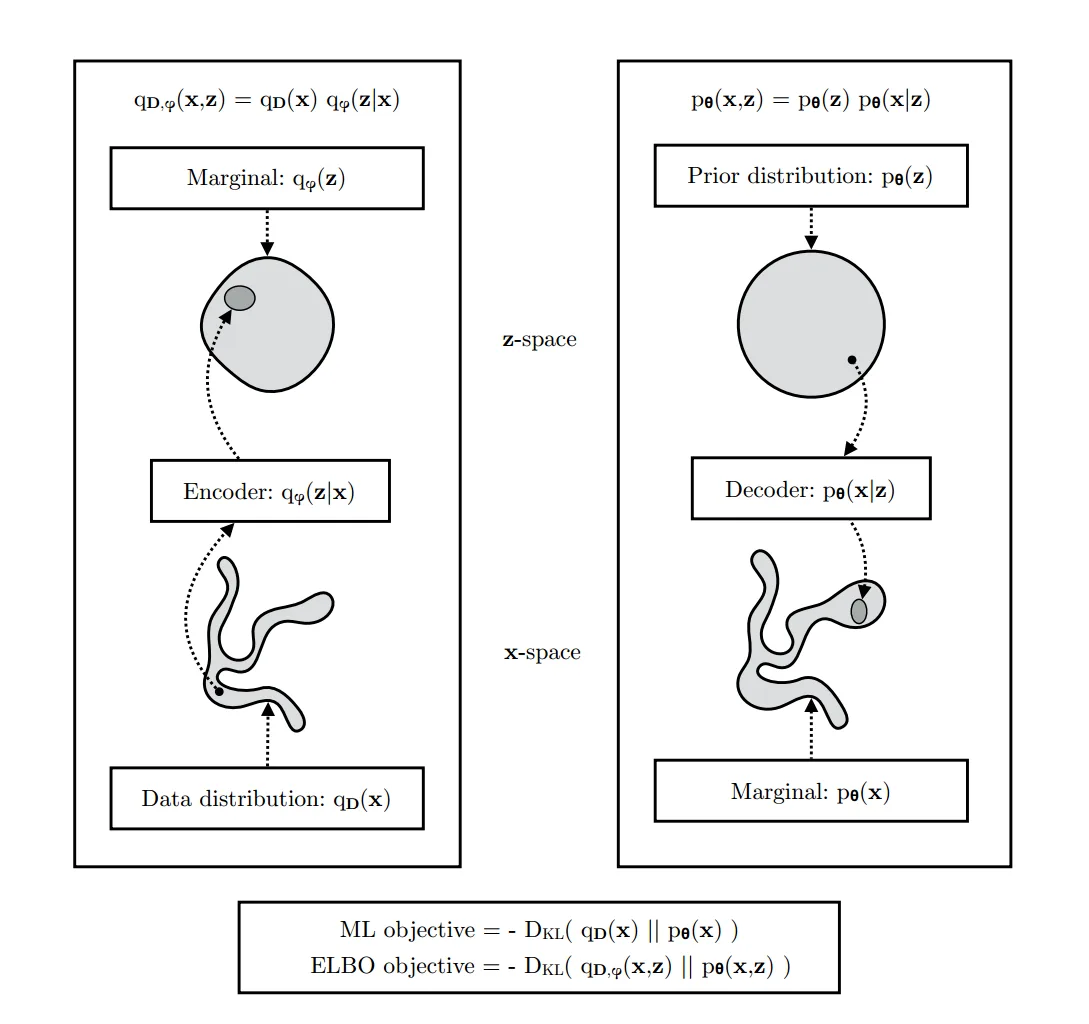
如果模型无法完美拟合，由于 KL 散度的方向，$p_\theta(\mathbf{x},\mathbf{z})$ 的方差通常会比 $q_{\mathcal{D},\phi}(\mathbf{x},\mathbf{z})$ 的方差大。

左图：编码过程。 数据 $\mathbf{x}$ 服从数据分布 $q_\mathcal{D}(\mathbf{x})$，经过编码器 $q_\phi(\mathbf{z}|\mathbf{x})$ 映射到潜空间，在潜空间中边缘化得到 $q_\phi(\mathbf{z})$。

右图：解码过程。 潜变量从先验 $p_\theta(\mathbf{z})$ 出发，通常取标准正态分布，经过解码器 $p_\theta(\mathbf{x}|\mathbf{z})$ 映射回数据空间，在数据空间中边缘化得到模型分布 $p_\theta(\mathbf{x})$。

Blurriness of generative model

上一节说过，优化 ELBO 相当于最小化 $D_{\text{KL}}(q_{\mathcal{D},\phi}(\mathbf{x}, \mathbf{z})||p_{\theta}(\mathbf{x}, \mathbf{z}))$。如果 $q_{\mathcal{D},\phi}(\mathbf{x}, \mathbf{z})$ 和 $p_\theta(\mathbf{x}, \mathbf{z})$ 不能完美匹配，那么 $p_\theta(\mathbf{x}, \mathbf{z})$ 和 $p_\theta(\mathbf{x})$ 的方差最终会比 $q_{\mathcal{D},\phi}(\mathbf{x}, \mathbf{z})$ 和数据分布 $q_{\mathcal{D}}(\mathbf{x})$ 的方差大。原因在于 KL 散度的方向。

如果某个 $(\mathbf{x},\mathbf{z})$ 在 $q_{\mathcal{D},\phi}$ 下有概率，而在 $p_\theta$ 下概率几乎为零，那么 $\mathbb{E}_{q_{\mathcal{D},\phi}(\mathbf{x}, \mathbf{z})} [\log p_{\theta}(\mathbf{x}, \mathbf{z})]$ 会趋于负无穷，惩罚非常大。反过来却不成立：生成模型在 $q_{\mathcal{D},\phi}$ 没有支撑的区域放一些概率，只会受到很轻的惩罚。所以模型倾向于把概率铺得更开，生成的样本看起来就比较模糊。

因此，选择足够灵活的推断模型和（或）生成模型，可以缓解这种模糊。